With the emergence of satellite position fixing systems, position determination at sea today has been reduced only to plotting of latitude and longitude read from the GPS screen display. Positions so obtained have very high level of accuracy, provided the equipment is working accurately. Radar and LORAN, where available are very frequently used navigational aids for position plotting.

However, the problem begins when too much reliance is laid on such aids. Navigators without the complete knowledge and understanding of traditional position fixing methods may find themselves handicapped in case of failure of the modern aids.

The principle philosophy of management of safety is, that every equipment that CAN FAIL and WILL DO SO and so the navigator must be prepared to use an alternate solution to navigation with total safety.

It is very important for every navigator to know methods of position fixing to be used under different circumstances, such as, poor visibility, limited availability of coastal features, coastal areas, deep ocean areas, tidal or non tidal areas, failure of Radar etc.

Navigation Chart position fixing methods are derived from geometrical theorems, which you have already learnt. While practising these techniques, you should relate to geometry for better understanding of these methods.

Position Line

The position line is the line on which the ship is most likely to be located. A bearing of a terrestrial object is a position line as the ship could be anywhere on that line. Since the distance from the object is not known, we cannot fix the position. However, it also must be noted that the bearing of a celestial object is not the position line as you would learn in the appropriate module, the position line in that cases is a line perpendicular to it. It is a position circle but for our purpose, the radius of the circle is so large that a tangent to the bearing can be accepted as a position line. There are more than one methods of obtaining position lines. Suppose you have found out the distance off an object, the arc of the circle with the radius, as the distance off becomes a position line. (Geometrically a position arc)

Position fixing by Horizontal Sextant Angle (HSA):

This method of position fixing is more suitable for ships at anchor or mooring, where accurate position determination is required and sufficient time is available. This method is based on the geometry theorem that angle subtended by any arc at the centre of the circle is twice the angle subtended at the circumference.

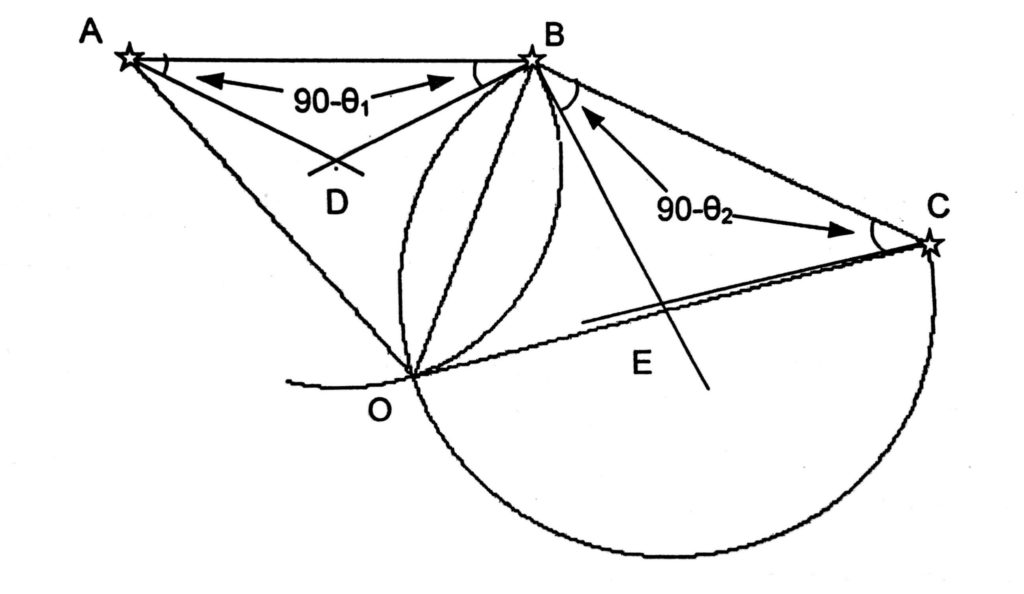
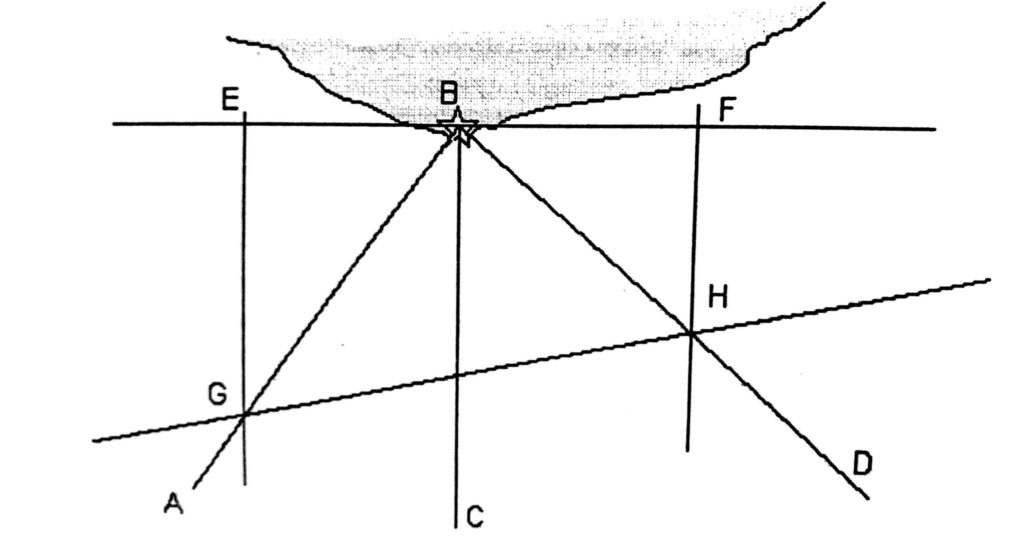
In above figure A, B & Care three identified charted shore objects. Using a sextant, measure a horizontal sextant angle (HSA). Between A and B let it be Ө₁ and between B & C Ө₂ .

Step 1. Join A & B and B & C by straight lines.

Step 2. Calculate the complement of the horizontal angle between A and B i.e. (90 — Ө₁ ). Plot it through A and again through B on the side towards the observer, giving intersection at point D. Similarly calculate and plot complement of HSA between B & C and plot the same through ‘B & C on the side towards the observer, giving intersection at point E.

Step 3. Using AD or BD as radius draw a circle with D as centre and also draw another circle using EB or EC as radius with E as centre. Position arcs AOB and BOG are part of position circles and the vessel lies on the intersection of the arcs at 0, as clearly ship cannot be on land at other intersection.

Advantages of horizontal sextant angle fixes,

1. It is more accurate because sextant can be read more accurately as compared to compass.

2. HSA fixes are free from compass error.

3. HSA can be taken from any part of the ship from where all the objects are visible. However, HSA fixes suffers from few drawbacks such as minimum 3 objects are required on or near a same straight line and more time is required for obtaining a fix.

Compass error determination

This method of position fixing can even be used for finding out compass error (gyro/standard) by joining the obtained fix on chart with any of the observed object by straight line and comparing this bearing on the chart with visually observed bearing.

Hence, even if compass error is not known three observed compass bearings of three objects can be used to obtain angle between objects and plotted as HSA in the similar manner. Compass error is obtained by comparing observed bearing and bearing obtained from the chart by joining the fix and object.

Position fixing by Vertical Sextant Angle (VSA).

In this method vertical sextant angle subtended by the object of known height (usually a lighthouse) is measured using a sextant, which gives distance off or position circle from the observed object. If more than one Vertical Sextant Angles (VSA) of nearby objects are observed simultaneously giving at least two position circles, intersection of such position circles will give the fix at the time of observation.

This again is not a very popular position fixing method used at sea as there are better and quicker methods of position fixing available. It is used in hydrographic surveys extensively. However, knowledge of these methods will prepare you for adverse situations, when usual methods of position fixing may not be available to you. You shall also be ready FOR solving it in the examinations without confusion. Remember index error needs to be applied.

This method of position fixing may suffer from the inaccuracy due to changing heights of observed objects from sea level caused due to tidal variations. Though these are difficult to calculate accurately the error that is likely to be caused is negligible and it is preferable to use the heights given the chart ad they are.

Method is found suitable for passing off- lying danger at a safe distance by sailing along an arc maintaining the pre-determined safe vertical sextant angle. Thus, any increase in the angle subtended at the observer indicates that the vessel is getting closer to the danger.

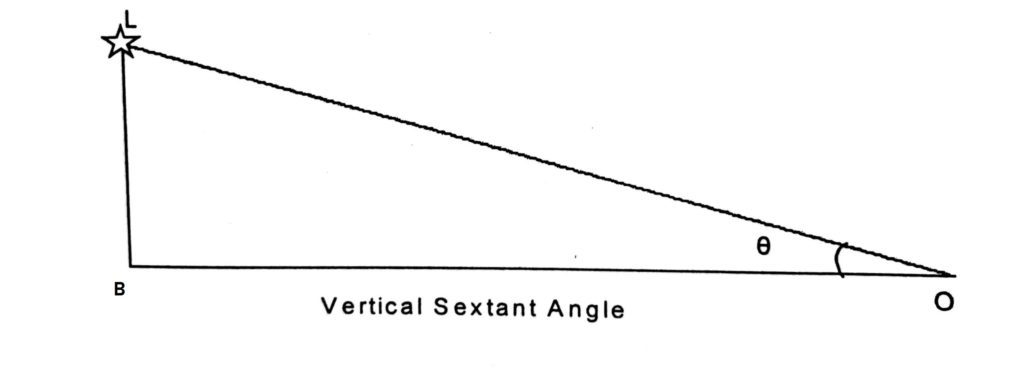
In the figure O is the observer on a ship and B is the base of a lighthouse at water level. L is the location of Lantern of the lighthouse.

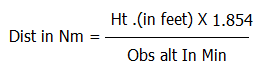
By using principles of trigonometry we know that BL = BO tan Ө.

As the angle Ө is small we can also say that BL = BO Sin Ө

i.e. Height = dist X Sin Ө

You are aware that at small angles, sine of an ” its angle is the same as radian. The value of one radian is 57° 17’45″= 3438 minutes.

Ө° = Ө / 57.3 radians

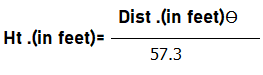
Therefore

Simplified this will become:

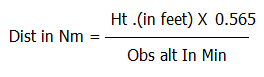
For objects in meters the formula becomes:

Running fix without current:

This method of position fixing is used when there is only one terrestrial object available for observing i.e., a lighthouse, light vessel whose position is known, without any means for measuring the distance from the object i.e. Radar out of order etc.

Running fix method uses the technique of transferring a position line. In this method, a position line is the observed bearing. Provided all conditions such as current, tide & wind etc. and the engine speed and course steered remains unchanged between the observations, the Position lines can be transferred for the short duration without much loss of accuracy.

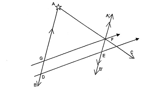
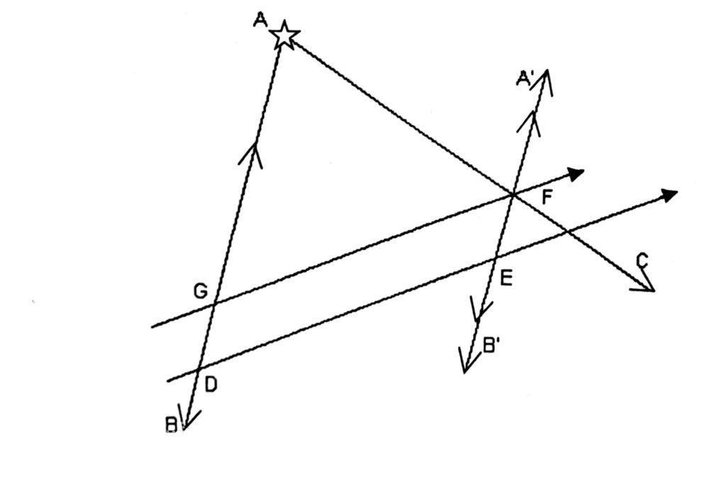
In the below figure, AB is the first observed bearing (position line). At the time of observation the vessel lay somewhere along this line If the vessel was steaming a course for a known period of time provided . all meteorological factors, engine speed, Course etc. remain unchanged, Line AB can be made to run for that period along the course steamed to A’ B’. Thus the vessel should now lie somewhere along A’ B’ which is a transferred Position line. (TPL).

We shall explain the method best, with the help of illustration given below:

While steering a course of 0700 (T) “A” Lt bore 014° (T) @1000 hours, and the same light bore 304° (T) @ 1030 hours, find the ship’s position at 1000 hours and @ 1030 hours. Speed by ship’s log 12 knots.

You can try this on an chart assuming a position for the given light and work on the same lines.

Follow the steps given below:

Step 1. Lay A B true bearing of Lt House @ 1000 hours i.e. 014°(T)

Step 2. Lay A C true bearing of Lt House @ 1030 hours i.e. 304° (T)

Step 3. AB being the position line @1000 hours, your vessel lies along this line. Take any point along AB, say, “D”. (Arbitrary position should be taken as close to DR as possible to minimise plotting error.)

Step 4. From D plot your true course being steered i.e. 0700 (T) and mark distance covered by your vessel between the interval of observations, 1000 hours to 1030 hours i.e. DE = 6 miles

Provided there were no changes in ship’s speed, course and prevailing meteorological conditions, position line of 1000 hours can be transferred through E without any loss of accuracy.

Step 5. Transfer position line AB through E i.e. A’ B’. Intersection of two position lines drawn is the ship’s position ‘F’ at 1030 hours. Now, if ship’s course is traced backward through F we get intersection “G”. This was the ship’s position at 1000 hours.

You may now ask as to what is the maximum duration for which a position line can be transferred. As stated earlier if speed and course other factors affecting the progress remain unchanged position lines theoretically can be transferred over a larger interval of time.

However, under normal circumstances a position line should not be transferred when navigating in the coastal waters for more than three hours.

Running fix with the current:

In case of simple running fix problem explained earlier ship’s speed and course are assumed unchanged during the interval between the observations. But in case of tidal areas where steady current of known strength and direction is experienced between the observations, following method is used for obtaining a fix.

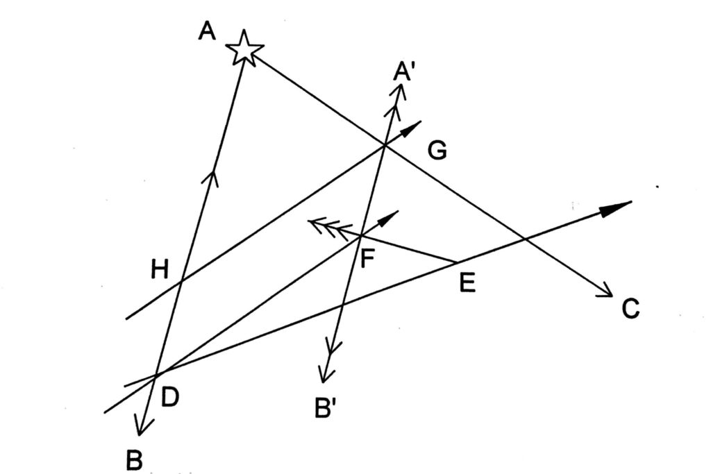
In our earlier illustration, of running fix, if vessel also experienced a tidal stream as setting 285 degrees at 3.5 knots, the working would be as follows:

Working is similar up to step 4.

Step 5. Draw set & drift vectors for 30 minutes through E up to F, i.e. 285 deg true and 1.75 Miles for interval of 30 minutes between 1000 hours and 1030 hours.

Step 6, Transfer Position line AB through F, intersection of A’B’ and AC at •G is the fix at 1030 hours and on tracing the course made good i.e. DF backward through G we get’ll’ fix at 1000 hrs.

Notice in this method course steered is not traced backward through ‘G’ instead course made good DF is drawn through ‘G’, to obtain position at 1000 hours.

You may wonder as to when and where am I really going to use these methods of position fixing in this era of satellite position fixing.

It just takes one complete black out or.a small accident or malfunctioning of system to spoil all the position fixing systems onboard and that is the time you need to put all your skills to use, for obtaining ship’s position accurately with limited means available to you. These position-fixing methods were devised in an era when such failures were common. They are not uncommon now either!

Three point bearing

Again, if you have no modem methods available and you have only one conspicuous object, it is possible to obtain a lot of information from three observations of the same object.

This is a very good method for obtaining course made good, using three observations of the same object taken at a known interval of time and therefore a known distance run between the observations.

Though there are various methods of calculating course made good, this method requires three bearings of only one object. Thus making it a very quick plotting method especially in coastal regions where the navigator I cannot afford to spare much time for plotting and needs to know accurately the course being made good by his vessel especially in cases of non availability of RADAR/ARRA /GPS etc.

Information needed is 3 bearings of any object taken at known interval of time and the distance steamed between those observations. This method is better illustrated stepwise as follows:

Step 1. Lay all three bearings AB, CB and DB through the observed object towards the sea.

Step 2. Through the observed object ‘IT, draw a line perpendicular to the middle bearing.

Step 3. On this line, mark the distance steamed between 1st and 2nd observation and the distance steamed between 2nd and 3rd bearing on their respective side of the middle bearing BE, BF.

Alternatively, instead of marking distances on the perpendicular line you may even mark the ratio of time or distance i.e. duration of 15 minutes and 45 minutes between the observations can be marked as 1:3. Distance steamed between observations of 4 miles and 16 miles can be marked as 1:4 using any suitable scale.

For this purpose, longitude scale is a very convenient scale as it is a constant scale and as we are not addressing the actual distances but their ratios.

Step 4. Draw lines parallel to the middle bearing i.e. EG & FH from the points obtained in step 3 on the either side of observed object till they meet first and third bearing and mark these two points ‘G’ and ‘H’ on the respective bearing.

Step 5. Join the points obtained in Step 4. GH is then the course made good between first and third bearing.

Primarily, this is not a position fixing method, however, if prevailing set is known fixes can be obtained at the time of 1st and 3rd bearing using running fix with current method as illustrated below:

Before proceeding further, please revise your running fix method again

Information needed is three bearings taken of a navigational object at a known interval of time or distance steamed between observation and set of the current.

 

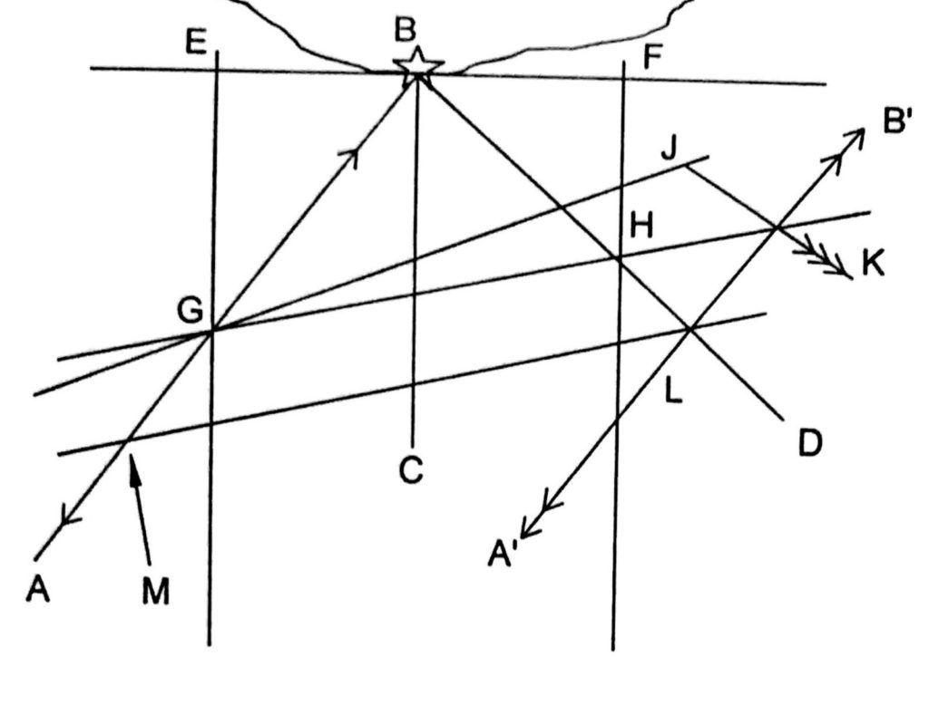
Step 1. Draw bearing AB, CB, DB through observed object towards the sea.

Step 2. Through B draw EF perpendicular to BC.

Step 3. Mark off EB & BF distance run between bearings or time or their ratio using a suitable scale on their respective sides.

Step 4. Through F & E draw FG & EH parallel to BC

Step 5. Join GH, being the course made good between the observations.

Step 6. Through ‘G’ draw course steered and mark ‘ at the distance steamed between the time interval of first and third bearing.

Step 7. Through J draw the direction of set experienced during the observation and extend it till it meets course made good at K.

Step 8. Through K draw A’B’, parallel to AB (transfer bearing AB through K) being the transferred position line at the time of third observation. Mark the intersection of A’B’ and DB (third observed bearing) ‘L.’

Step 9. ‘L’ is the ship’s position at the time of third bearing observation. Transfer GH through `L’ in reverse direction, from intersection of transferred course made good and first bearing gives you ship’s position ‘M’ at the time of first observation.

Step 10. JK is the drift experienced during the interval between first and third observation.

Doubling the angle on the bow for obtaining the distance off.

In the figure ‘C’ is a lighthouse being observed. When taking first bearing, the time and log reading is noted down, the observer continues to observe the light-house till the observed bearing becomes double in value on the bow (relative bearing on port or starboard bow). Time and speed log is noted to calculate distance steamed between these two observations.

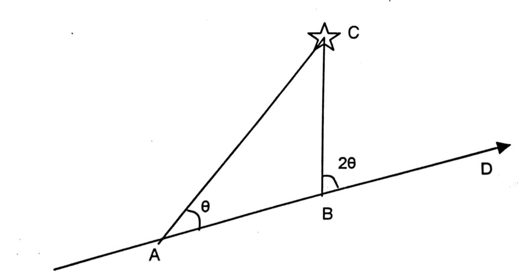
AC — first bearing of light

BC — Second bearing of light

AD — Course steered between observations.

AB = BC = Distance run between first and second observations

BC — Distance from the light at the time of second observation

In this illustration, initial relative bearing on port bow was the ∠BAC = Ө° and at the time of second observation relative bearing an bow ∠CBD = 2Ө.

Distance steamed between first and second observation is the distance from observed object, (in this case lighthouse) because triangle ABC is isosceles triangle with AB = BC.

This method gives distance from the object observed at the time of second observation. It does not help in predicting or planning distance off in advance.

Four point bearing on the bow for knowing the distance off.

The procedure is similar to doubling the angle on bow. When angle on bow is equal to four points, (i.e. 11.25° x 4 = 45°) note down time and log and continue to observe the object till the angle on the bow becomes 90° (11.25° x 8 = 90°). Distance from the object shall be the distance steamed between first and second observation.

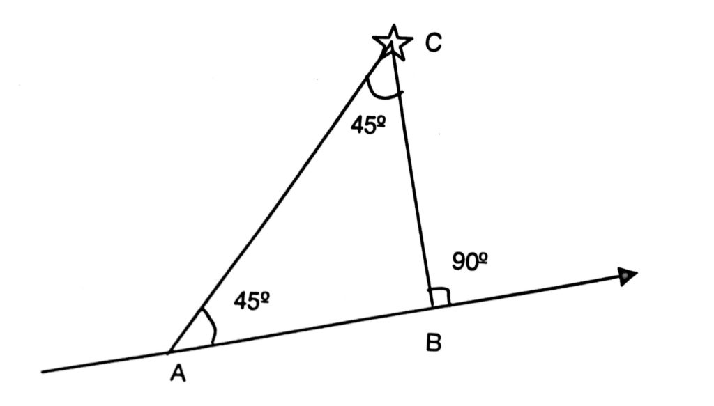
AC = first observation, when angle on the bow is 45°.

BC= second observation, when angle on the bow is 90°. AB = BC.

This method also suffers from the disadvantages that distance from the object is only known when ship is already off that position.

Special angles on the bow.

We use this process for estimating the distance abeam, at which the ship is going to pass any observed object. Special angle method of estimating distance gives the distance abeam from the object in advance, enabling us to take a decision regarding safe passing distance etc.

Unlike doubling the angle on the bow or four point bearing methods, if certain pairs of angles (table A) are observed on the bow and time and log is noted, distance off When abeam can be estimated.

A pair of selected angles are observed on the bow whose cotangent value gives difference of one, thus the distance steamed between two observations will be the distance off, when vessel is abeam the target.

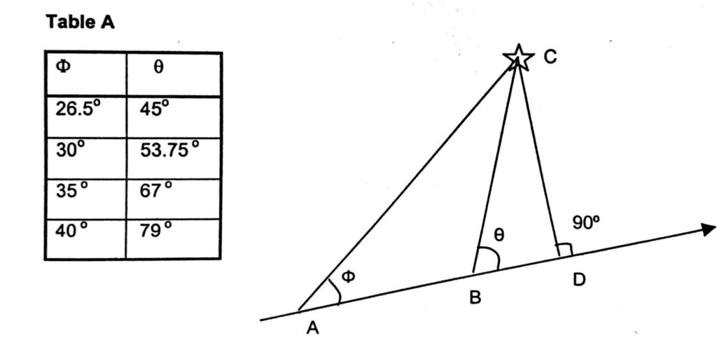
AD = ship’s course steered

AC = first relative bearing such as ∠ BAC= Φ (any special angle from tableA)

BC = second relative bearing such as ∠ DBC = Ө (paired special angle with first angle on the bow)

From figure

Cot Ө = BD/DC ———–(1)

Cot Φ = (AB+BD) / DC= (AB/DC)+(BD/DC)

From (1) and (2)

Cot Φ – Cot Ө = (AB/BC) +(BD/DC) — (BD/DC) = (AB/DC)

Cot Φ – Cot Ө = (AB/DC)

If AB = DC
AB/DC = 1

Hence, Cot Φ – Cot Ө =1

A good number of pairs will fulfil this requirement. More frequently used pairs are given in Table A.

Range of navigational lights

Visibility range of any navigational lights can be defined in three following ways.

1. Geographical range

2. Luminous range, and

3. Nominal range

Geographical range

Geographical range is the maximum distance at which a light can be seen considering the height of the light and height of the observer’s eye, due to curvature of the earth surface. This range in sea miles can be directly obtained from the table provided in the Admiralty list of lights. Geographical range can also be calculated by using visible horizon formula given below:

Due to curvature of earth’s surface visibility, range of lights depends upon various factors i.e. the height of the light, height of the observer’s eye, intensity of the light and the prevailing visibility.

• Higher the observer, larger is the visible horizon.
• Higher the location of light, larger is the visible horizon.
• Higher the intensity of light, farther it is visible.
• Better the atmospheric visibility, farther the visible range.

Imagine yourself onboard a large tanker. During your loaded passage, your height of eye will be less as compared to the height of eye on ballast voyage. Hence, will see lights much later as compared to ballast voyage. Similarly, lighthouses located on higher islands or taller structures would also be visible much earlier as compared to the lights of less height. In addition to the height and intensity of the light, atmospheric visibility also governs the visible range of any light.

Step 1. Find out the height of the lighthouse from chart or Admiralty list of lights and fog signals and calculate the range of visible horizon of the light using following expressions.

Distance of visible horizon = 1.15 x  √ h (h = height of light house or observer in Feet)

Distance of visible horizon = 2.095 x  √ h (h = height of light house or observer in Meters).

Step 2. Calculate height of eye (HE) of the observer (HE corresponding to draft is displayed on the bridge) and calculate the range of visible horizon for the observer using formula given in step 2

Step 3. Add range of visible horizon for observer and that of lighthouse. This sum gives you the maximum range at which the observer and the lighthouse will be in the line of sight.

This range is called as geographical Range

Luminous range

Luminous range is the maximum distance at which a light can be seen in the prevailing visibility conditions due to the intensity of light alone. This range does not consider the curvature of earth, elevation of light, and observer’s height of eye.

Luminous range diagram is provided in the Admiralty list of lights and fog signals and from the table luminous range can be worked out for any light of known intensity in candelas.

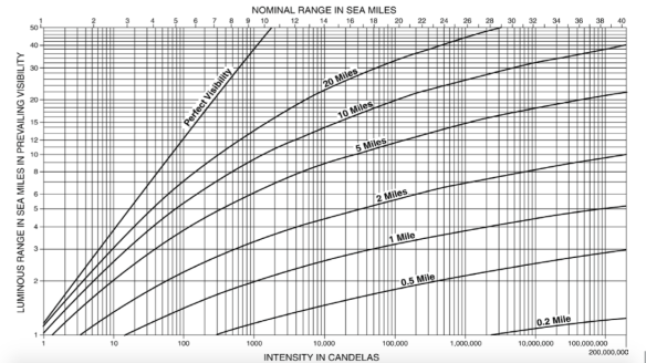
Nominal Range

It is the maximum range at which a light can be seen in the prevailing visibility of 10 nautical miles, or It is the luminous range of any light in the meteorological visibility of 10M.

Ranges marked in charts and in list of lights are normally luminous or nominal ranges .To know the type of the range, reference should be made in the special remark column of list of lights or cautions given on the navigational charts. in the absence of any information, for all practical purposes ranges marked on the chart are taken as luminous range.

Thus, the maximum range at which a light will be visible will either be geographical or luminous range whichever is less.

It is necessary to calculate both ranges to determine the visible range of the light.

Example – 2

Assuming your height of eye is 16m, calculate at what range will the light be sighted. Elevation of light is 20 m. Other details are the same as in example 1 Follow me:

Step 1. Calculate visible horizon of the observer and of lighthouse as explained earlier or using geographical range tables from list of lights.

Step 2. Calculate geographical range of the lighthouse by adding both the ranges.

Step 3. Compare charted range and the calculated geographical range A light will be seen at the lesser of the two ranges.

The geographical range is sometime more than the charted range. This is because though the elevation of light and observer’s height of eye gives a larger range insufficient power of the light rates the charted range at a lower range. Such lights cannot normally raised or dipped.

Some lights have a very large luminous range but their geographical range is limited due its height. The loom of these lights can be seen at very large distances but they are raised at the rising distances only.

Raising and dipping of lights

A light is raised when it is seen on the horizon from the bridge of a ship for the first time. A light is dipped when the light is seen for the last time on the horizon from the ship as the ship goes away from the light. Rising and dipping distances of the light are the maximum visible ranges. We can calculate these distances using formulae or range tables. Rising and dipping bearings and distances can give us reasonably accurate fixes. However, positions thus obtained must be used with caution, as distances off (rising or dipping distances) may not be very accurate.